If you deal with Excel regularly, then you are probably searching for a quick and easy way to add immediate visual clarity to your spreadsheets. Many Excel files include large amounts of data which are not arranged or presented in any useful graphic fashion.
The conditional formatting tool assists you to read the Excel workbook, identify key items and present to others in a manner that few other methods can do so effectively and easily.
Purpose
Microsoft Excel’s Conditional Formatting feature allows the user to highlight, color, and apply other formatting preferences to a group of cells, based on certain criteria. It immediately transforms a jumble of data into useful information in a visual and aesthetically pleasing manner.
Why use it?
The image of the highlighted and formatted cells adds instantaneous clarity for both the user and the viewers. You can identify outliers and problem areas quickly.
Limitations
The Conditional Formatting feature is only as helpful and intuitive as the user, who must input all required criteria to maximize the functionality of the feature. The text amidst numbers may be formatted awkwardly.
Example and Steps to Follow
You’ve just started a new job at Food Mood, a small local grocery. The owner voices how he is losing money due to inventory being wasted and thrown out as a result of overstocking and expirations. You are tasked with managing the logistics of ordering and stocking food.
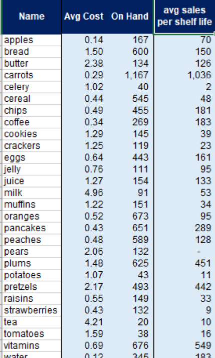
Fortunately, you’ve got great data collected for you by the previous accounting professional. Here are their raw numbers compiled for you.
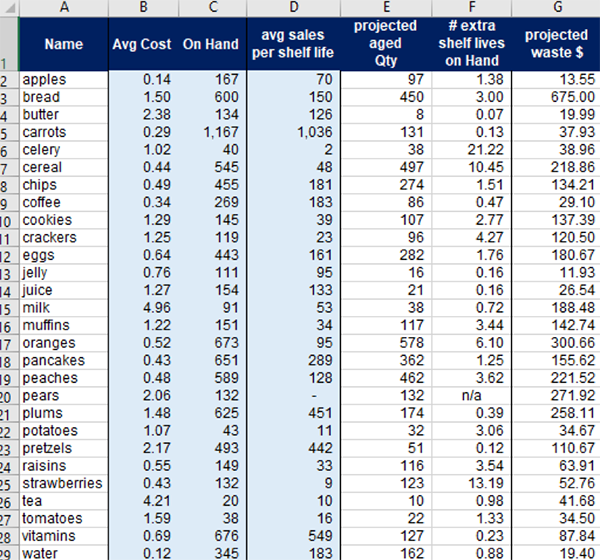
Utilizing some basic formulas, you create the following, which translates the raw data into projected dollar-values for food which will expire next Monday.
Now to identify the key problem items. If you’re thinking a simple sort will provide the answer, then you are correct in this instance. Sorting column G largest-to-smallest will identify the biggest waste dollars.
But, sorting is not always the best solution. Let’s bring in conditional formatting!
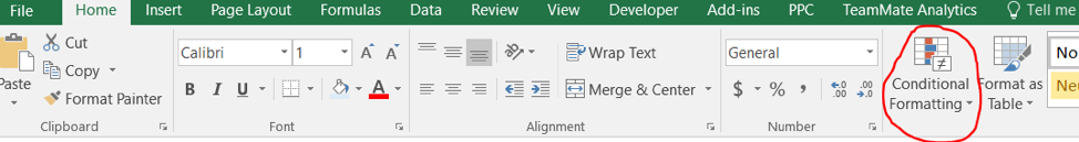
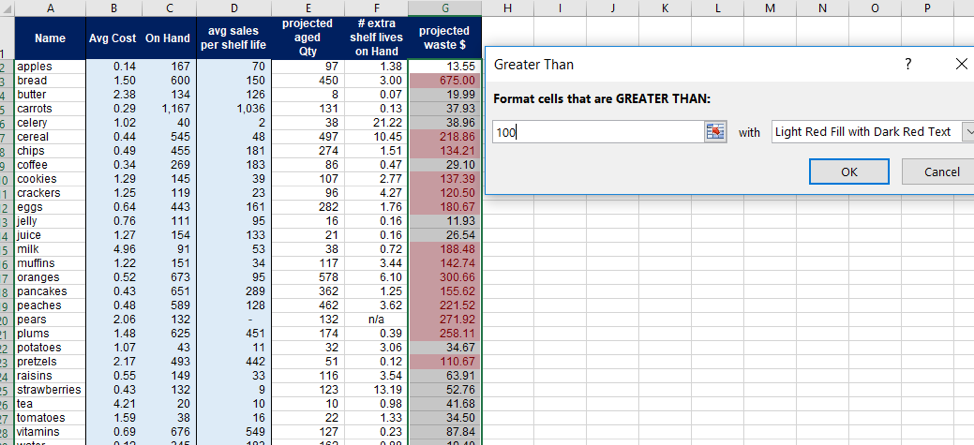
Highlight the cells upon which you want to apply the formatting (Column G). Click the circled image above and a drop down with a wide variety of potential criteria at your arsenal will appear. In this case, the owner only wants to investigate wastes above $100 per shelf life. Hover over “highlight cells” and input that as your criteria. Select “greater than”, and then, put in the amount. The data automatically formats to show you the result.
You have pressed OK, and you’re still looking for more clarity. For some items, our vendors can only provide the shipments in bulk, such that we cannot tailor the exact order amount we want. Since the sales are always increasing, we do want at least some bulk. That leads you to the next step:
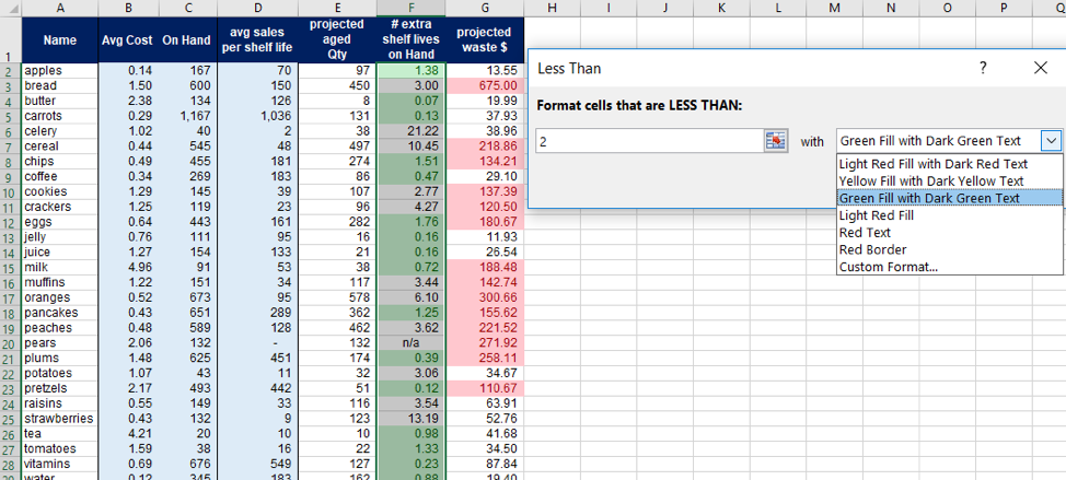
2. Some products are overstocked by more than double their lives. That’s a problem! Which items have less than double their lives’ on-hand quantities? Select the cells, modify your criteria to be less than, and choose a new “happier” color which indicates these are not problem items:
Done! One more problem to go.
The owner has indicated that too much variety in this small store is leading to logistics confusion and adding to waste. As such, he wants to get rid of all products for which sales are less than 50 units per shelf life.
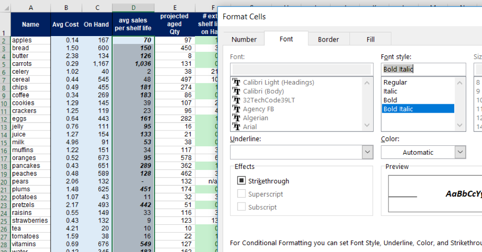
Our picture is beginning to look like art. Let’s use a different formatting type. The “custom format” will open up additional endless opportunities with which we can express certain cells’ values.
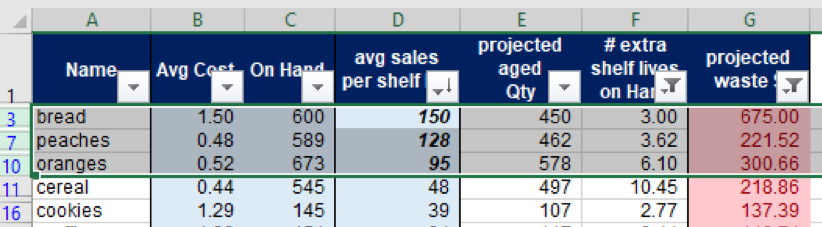
Through applying filters by cell style, you have come up with the only major problem items based on all the information above.
Additional items to keep in mind:
- Formats can be set on top of other formats to achieve layered conditional formatting.
- Clearing formats can be done with “clear rules from cells” found in the initial drop-conditional formatting down menu.
- In this example, we only explored the highlight cells feature within conditional formatting. Play around in the initial drop-down menu for the other useful tools!
Taking it to the next level:
Once you have experimented with this functionality, you will discover that Excel’s capabilities with this feature are wide-reaching. Cells can be formatted based on formulas, based on other cells, based on text and dates, and many more. As always, there are multiple methods by which to accomplish your desired result in Excel.
Have fun with it and keep expanding your Excel prowess!
You may also like: